Tutorial 1: Generating surrogate maps on the cortex

In this first example, we will derive a set of surrogates for the gradient data we covered in the Getting Started section. We will use this set of surrogate data to statistically compare two brain maps. This process will give us a correlation metric and a means by which to test the significance of the association between them.

Nulls with surface data

We’ll first start by loading the Allen Human Brain Atlas gene PC1 and everything we need to compute the surrogates:

>>> from eigenstrapping import datasets, fit
>>> genepc_lh, genepc_rh, emodes_lh, emodes_rh, evals_lh, evals_rh = datasets.load_surface_examples()
>>> distmat, index = datasets.load_distmat('fsaverage', hemi='lh', sort=True)
>>> # note: this download may take a while
>>> surrs_lh = fit.surface_fit(
                    x=genepc_lh,
                    D=distmat,
                    index=index,
                    emodes=emodes_lh,
                    evals=evals_lh,
                    num_modes=100,
                    nsurrs=1000,
                    resample=False,
                    return_data=True,
                    )
No surface given, expecting precomputed eigenvalues and eigenmodes
IMPORTANT: EIGENMODES MUST BE TRUNCATED AT FIRST NON-ZERO MODE FOR THIS FUNCTION TO WORK
Surrogates computed, computing stats...

>>> surrs_lh.shape
(1000, 10242)

Those who’ve completed the Getting Started section might notice that we’re not using the eigenstrapping.SurfaceEigenstrapping class anymore, but the eigenstrapping.fit module now. This module allows us the same control over the parameters as before, but it also gives us an output variogram and other helpful info. The above code will give you a figure:

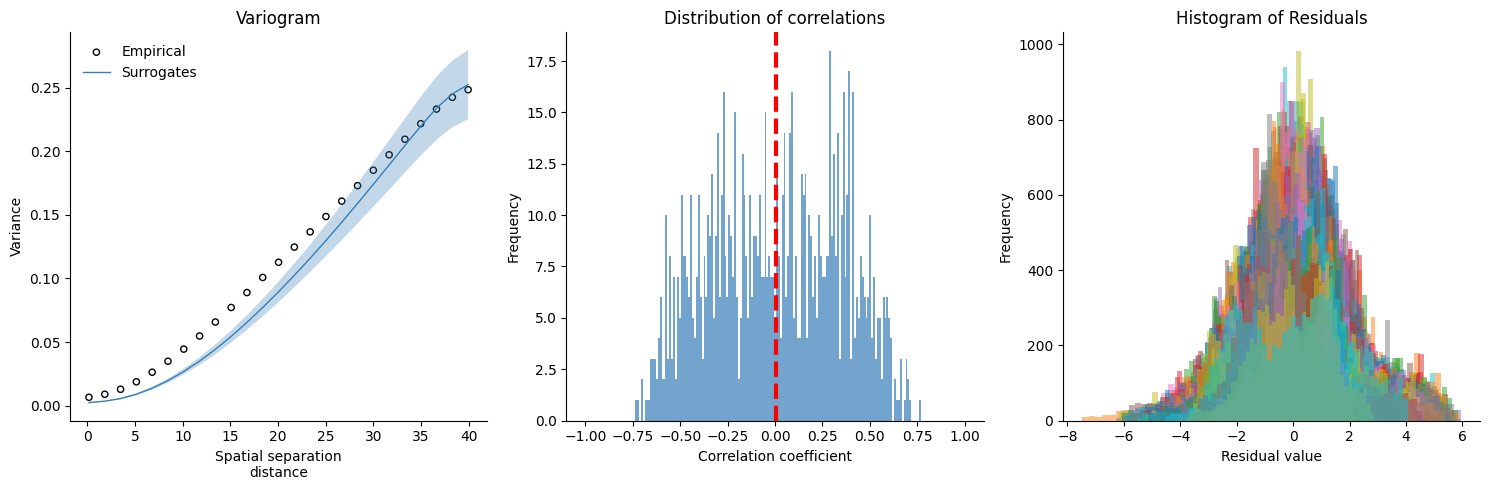
We can see that the variogram of the surrogates doesn’t match up with the empirical data (they’re too smooth, hence a lower variogram curve). The residuals in the third plot also don’t form a low amplitude Gaussian, meaning they have some information in them. It is worth noting here that the residuals may never form a low amplitude Gaussian. It depends on the structure of the original data, and if that data is highly non-normal. Hence why we perform non-parametric statistics in the first place.

To form a proper null, the surrogates should line up with the empirical variogram. We need to increase the number of modes that we use:

>>> surrs_lh = fit.surface_fit(
                        x=genepc_lh,
                        D=distmat,
                        index=index,
                        emodes=emodes_lh,
                        evals=evals_lh,
                        num_modes=250,
                        nsurrs=1000,
                        resample=False,
                        return_data=True,
                        )
No surface given, expecting precomputed eigenvalues and eigenmodes
IMPORTANT: EIGENMODES MUST BE TRUNCATED AT FIRST NON-ZERO MODE FOR THIS FUNCTION TO WORK
Surrogates computed, computing stats...

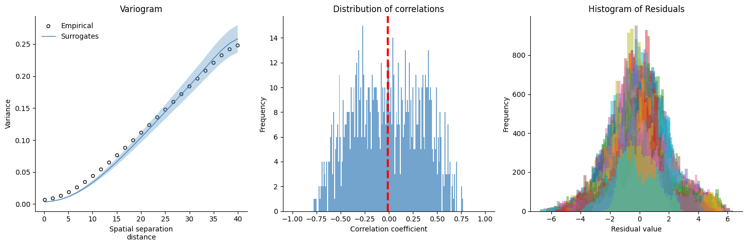
250 modes seems to be a better fit for the gene PC1 data. You may notice that the surrogate distribution is now wider, better reflecting the underlying null.

Let’s compare the gene PC1 map to another brain map, now that we’ve generated the null distribution:

>>> from eigenstrapping import stats
>>> from neuromaps import datasets as ndatasets, transforms, images
>>> neurosynth_lh = images.load_data(
    transforms.mni152_to_fsaverage(
        ndatasets.fetch_annotation(source='neurosynth', return_single=True),
        fsavg_density='10k'
    )
)[:10242] # download and load the neurosynth principal gradient, we only want the left hemisphere
>>> corr, pval, perms = stats.compare_maps(genepc_lh, neurosynth_lh, nulls=surrs_lh, return_nulls=True)
>>> print(f'r = {corr:.3f}, p = {pval:.3f}')
r = 0.350, p = 0.401

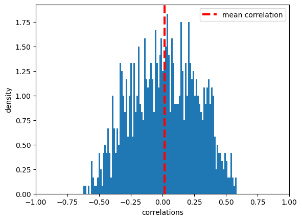
We can also plot the histogram of null correlations to the target map to make sure it is what we expect (the mean value of correlations should be ~0), while the distribution should follow a roughly-Gaussian shape

>>> import matplotlib.pyplot as plt
>>> plt.hist(perms, bins=101, density=True)
>>> plt.xlim([-1, 1])
>>> plt.axvline(perms.mean(), linestyle='dashed', zorder=3, lw=3, color='r', label='mean correlation')
>>> plt.xlabel('correlations')
>>> plt.ylabel('density')
>>> plt.legend(loc=0)
>>> plt.show()

Make sure that the first argument of the stats.compare_maps function is the map that the surrogate array was computed on, otherwise you can get strange behavior.