Meshes and mesh operations

Remeshing

Sometimes it is useful to remesh a triangular surface as a tetrahedral mesh and vice-versa - say, if one wants to derive 3D surfaces within subcortex. This routine is implemented within the eigenstrapping.geometry.remesh() function, which automatically recognizes the surface type (triangles or tetrahedra) and maps the surface to the other type.

For example, you have a hippocampal volume in MNI152 space (we can load this from the eigenstrapping.datasets.fetch_data() function), you can remesh it from a volume to a triangular mesh. By default these will be generated in the same folder that the original volume/mesh is in.

>>> from eigenstrapping.datasets import fetch_data

>>> hipp_lh = fetch_data(
                name='brainmaps',
                hemi='lh',
                format='hippocampus'
                )
>>> hipp_lh
'/mnt/eigenstrapping_data/brainmaps/space-MNI152_res-2mm_hemi-lh_hippocampus.nii.gz'

>>> from eigenstrapping.geometry import remesh

>>> hipp_tria_lh = remesh(hipp_lh)
>>> hipp_tria_lh
'/mnt/eigenstrapping_data/brainmaps/space-MNI152_res-2mm_hemi-lh_hippocampus.tria.vtk'

You can also remesh from a triangular mesh to a tetrahedral one:

>>> hipp_tetra_lh = remesh(hipp_tria_lh)
>>> hipp_tetra_lh
'/mnt/eigenstrapping_data/brainmaps/space-MNI152_res-2mm_hemi-lh_hippocampus.tria.tetra.vtk'

Deriving eigenmodes from a mesh

Deriving LBO vector solutions to the Helmholtz equation, or eigenmodes as we refer to them, is a fairly trivial process once a mesh has been defined. As graph representations of meshes are sparse by their very nature (on a triangular mesh, a single vertex only ever has three edges at the most; four in a tetrahedral mesh), we can use sparse methods of deriving these modes.

We use the finite element method as implemented in ShapeDNA, the details of which can be found in the requisite papers in References. The form matrices, A and B, are derived either through Cholesky decomposition using the scikit-sparse libraries, or LU decomposition in scipy.sparse.splu if the former is not installed. We recommend, if possible, to install the scikit-sparse libraries as Cholesky decomposition is much faster than LU.

Let’s take our remeshed tetrahedral hippocampus and use eigenstrapping.geometry.calc_eig():

>>> from eigenstrapping import geometry
>>> tetra = geometry.load_mesh(hipp_tetra_lh)
>>> # in this case, we'll use eigenstrapping.geometry.calc_eig without sksparse
>>> emodes, evals = geometry.calc_eig(tetra, num_modes=20)
TetMesh with regular Laplace
Solver: spsolve (LU decomposition) ...

>>> # by default, this function will remove the first (constant) mode
>>> # this behavior can be changed by setting `return_zero=True` in
>>> # the calc_eig function

>>> emodes
array([[ 0.01210057,  0.01249517,  0.00465954, ..., -0.00146934,
        -0.00544099,  0.0271714 ],
       [ 0.01209385,  0.01253431,  0.00548657, ..., -0.00434336,
        -0.00504929,  0.0242422 ],
       [ 0.01198019,  0.01202892,  0.00418164, ..., -0.00095343,
        -0.0038022 ,  0.02745249],
       ...,
       [-0.00412068, -0.01866016,  0.00250916, ...,  0.00476944,
        -0.00805506, -0.00263126],
       [ 0.00052041, -0.01061745, -0.00131715, ...,  0.00542975,
        -0.00041589,  0.01133534],
       [-0.01403812, -0.0024371 ,  0.00991763, ...,  0.02579329,
        -0.02810065,  0.00869789]], dtype=float32)

>>> evals
array([0.00365112, 0.01341067, 0.02674828, 0.03218102, 0.04489195,
       0.05093223, 0.06653866, 0.07089102, 0.09374754, 0.09695608,
       0.10020526, 0.11701339, 0.12567881, 0.13450024, 0.14623912,
       0.15450524, 0.15965985, 0.16787478, 0.17781733, 0.18272817],
      dtype=float32)

>>> # as you can see, the first column of `emodes` is not constant.

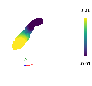
Now, let’s plot the first non-constant eigenmode on the surface of the mesh.

>>> from eigenstrapping import plotting

>>> plotting.meshplot(hipp_tetra_lh, emodes[:, 0], vrange=0.01, colorbar=True)

Mesh distance calculations

We also provide geodesic (surface) and Euclidean (volumetric) distance calculations for meshes. Geodesic distance calculation is performed using a heat kernel on each vertex, and takes about 2 hours for a 32k standard hemisphere (fsLR). See the paper in References for specific details on the implementation.

In order to calculate the geodesic distance matrix, we use the eigenstrapping.geometry.geodesic_distmat() function, which takes an input mesh:

>>> from eigenstrapping import datasets

>>> surf_lh, *_ = datasets.load_surface_examples(with_surface=True)
>>> surf_lh
'/mnt/eigenstrapping-data/surfaces/space-fsaverage_den-10k_hemi-lh_pial.surf.gii'

>>> # for our purposes, we won't use sksparse libraries, but to do so, we
>>> # pass `use_cholmod=True` to the function
>>> distmat_lh = geometry.geodesic_distmat(surf_lh, use_cholmod=False)
# eventually ...

>>> distmat_lh.shape
(10242, 10242)

>>> distmat_lh
array([[  0.        ,  91.41330719,  73.28165436, ..., 184.62254333,
        186.47727966, 187.92669678],
       [ 91.41330719,   0.        ,  81.62067413, ..., 127.93047333,
        129.78521729, 131.2346344 ],
       [ 73.28165436,  81.62067413,   0.        , ..., 114.22114563,
        116.07588959, 117.52529907],
       ...,
       [184.62254333, 127.93047333, 114.22114563, ...,   0.        ,
          2.80057883,   4.78903866],
       [186.47727966, 129.78521729, 116.07588959, ...,   2.80057883,
          0.        ,   1.98845983],
       [187.92669678, 131.2346344 , 117.52529907, ...,   4.78903866,
          1.98845983,   0.        ]])

You can speed things up in the eigenstrapping.geometry.geodesic_distmat() function by passing n_jobs=<number of workers>. For instance, to use eight threads, you would pass n_jobs=8. To use every available thread, pass n_jobs=-1.

Euclidean distance calculation is performed in a similar way:

>>> distmat_lh = geometry.euclidean_distmat(mesh) # much quicker than geodesic
>>> distmat_lh.shape
(10242, 10242)

>>> distmat_lh
array([[ 0.        , 54.72087326, 37.01728554, ..., 94.95060009,
        93.16259385, 92.16275463],
       [54.72087326,  0.        , 61.99785175, ..., 98.85110323,
        98.2701815 , 98.01616578],
       [37.01728554, 61.99785175,  0.        , ..., 78.64858645,
        77.51088511, 77.12512891],
       ...,
       [94.95060009, 98.85110323, 78.64858645, ...,  0.        ,
         2.80057878,  4.7547238 ],
       [93.16259385, 98.2701815 , 77.51088511, ...,  2.80057878,
         0.        ,  1.98845989],
       [92.16275463, 98.01616578, 77.12512891, ...,  4.7547238 ,
         1.98845989,  0.        ]])

Notice the pronounced difference between the two methods. This is because the cortex is constructed as a 2D sheet (basically the surface of a sphere), so it is not advisable to use Euclidean distance calculations. For the subcortical volumes, you would use the Euclidean distance.